Quickstart
Suppose we want to solve the integro-differential equation (IDE)
The analytic solution to this IDE is \(y(x) = \ln(1 + x)\). We’ll find a numerical solution using IDESolver and compare it to the analytic solution.
The very first thing we need to do is install IDESolver. You’ll want to install it via pip (pip install idesolver) into a virtual environment.
Now we can create an instance of IDESolver, passing it information about the IDE that we want to solve.
The format is
so we have
In code, that looks like (using lambda functions for simplicity):
import numpy as np

from idesolver import IDESolver

solver = IDESolver(
    x = np.linspace(0, 1, 100),
    y_0 = 0,
    c = lambda x, y: y - (.5 * x) + (1 / (1 + x)) - np.log(1 + x),
    d = lambda x: 1 / (np.log(2)) ** 2,
    k = lambda x, s: x / (1 + s),
    f = lambda y: y,
    lower_bound = lambda x: 0,
    upper_bound = lambda x: 1,
)
To run the solver, we call the solve() method:
solver.solve()

solver.x  # whatever we passed in for x
solver.y  # the solution y(x)
The default global error tolerance is \(10^{-6}\), with no maximum number of iterations. For this IDE the algorithm converges in 40 iterations, resulting in a solution that closely approximates the analytic solution, as seen below.
import matplotlib.pyplot as plt

fig = plt.figure(dpi = 600)
ax = fig.add_subplot(111)

exact = np.log(1 + solver.x)

ax.plot(solver.x, solver.y, label = 'IDESolver Solution', linestyle = '-', linewidth = 3)
ax.plot(solver.x, exact, label = 'Analytic Solution', linestyle = ':', linewidth = 3)

ax.legend(loc = 'best')
ax.grid(True)

ax.set_title(f'Solution for Global Error Tolerance = {solver.global_error_tolerance}')
ax.set_xlabel(r'$x$')
ax.set_ylabel(r'$y(x)$')

plt.show()
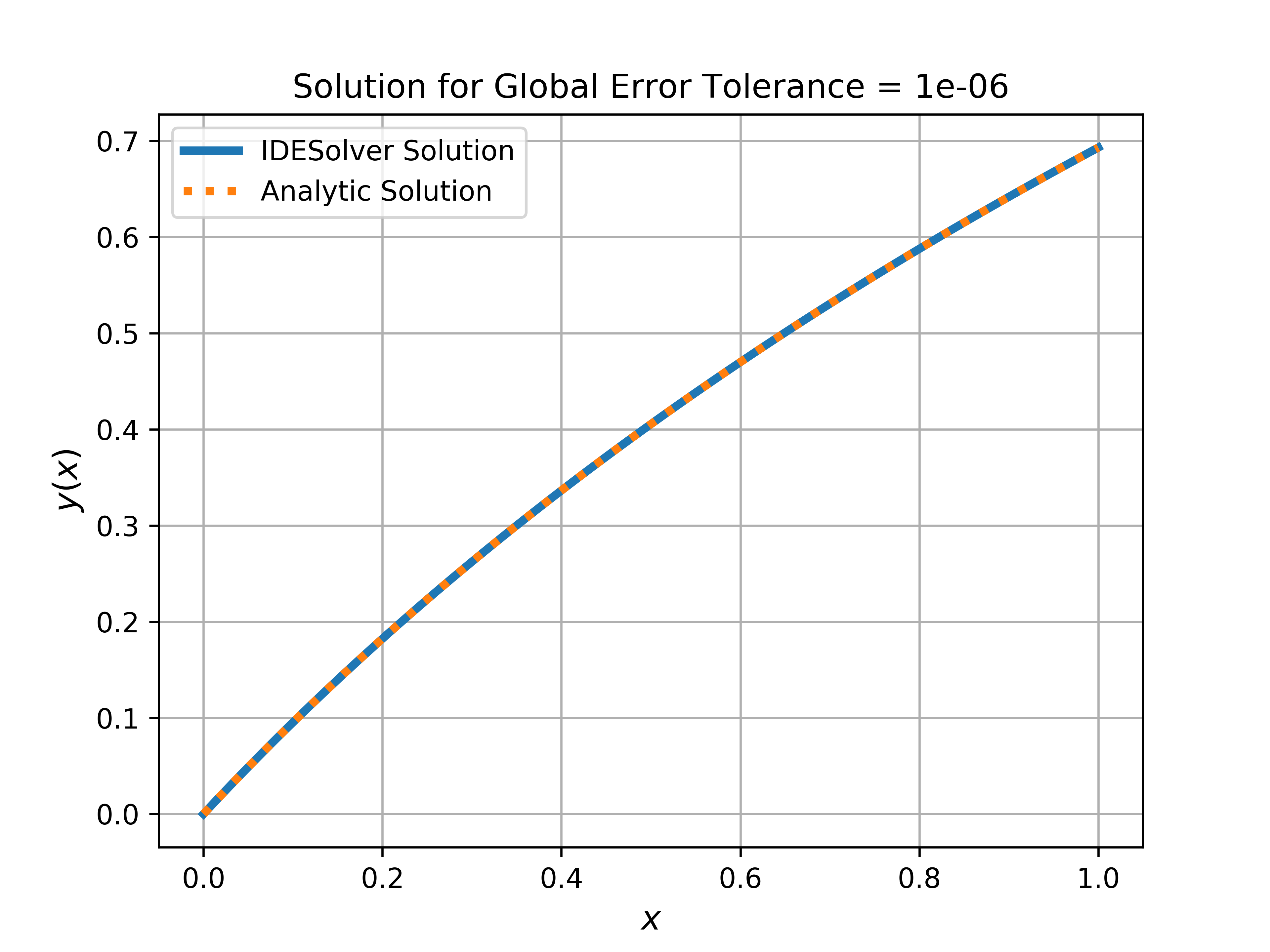
fig = plt.figure(dpi = 600)
ax = fig.add_subplot(111)
error = np.abs(solver.y - exact)
ax.plot(solver.x, error, linewidth = 3)
ax.set_yscale('log')
ax.grid(True)
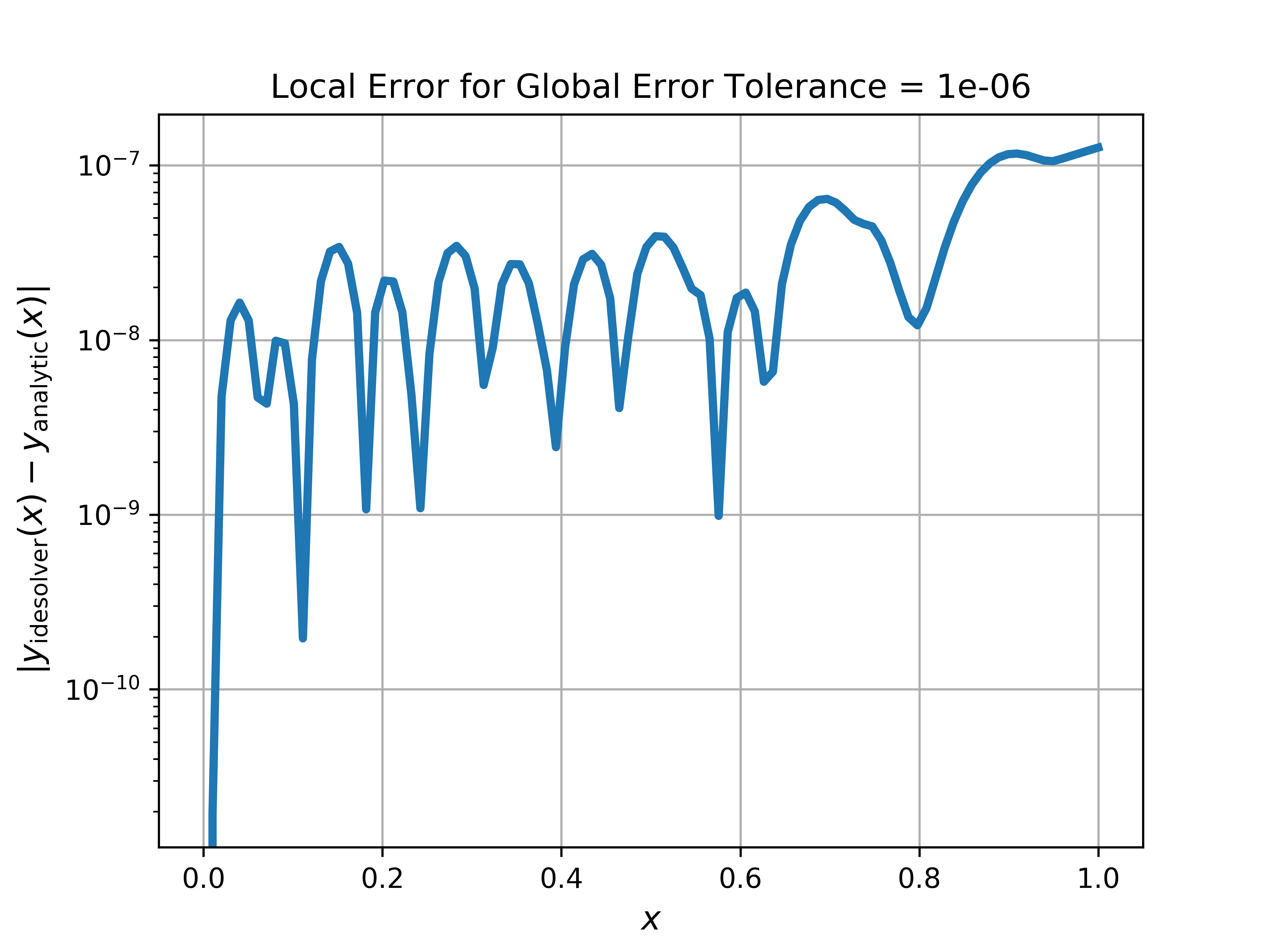
ax.set_title(f'Local Error for Global Error Tolerance = {solver.global_error_tolerance}')
ax.set_xlabel(r'$x$')
ax.set_ylabel(r'$\left| y_{\mathrm{idesolver}}(x) - y_{\mathrm{analytic}}(x) \right|$')
plt.show()